Paper——LeGO LOAM

LeGO LOAM: Lightweight and Ground-Optimized Lidar Odometry and Mapping on Variable Terrain.

• real-time performance in embedded device
• more robust when facing challenging case
• reduced computational expense ### Pipeline

Untitled

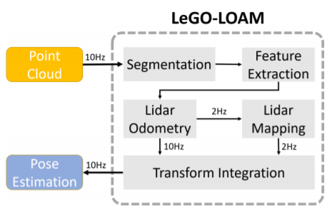
Lidar odometry: local pose (fast but inaccurate)

Lidar mapping: register current pcd into the global map (slow but accurate)

Segmentation

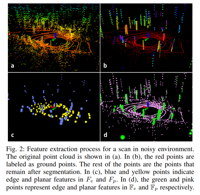
Segmentation is a pre-processing before odometry, to remove unreliable points and distinguish ground points and other points.

1. First the point cloud will be projected onto a range image （1800 * 16, because the lidar has a vertical fov of 30° and horizontal fov of 360°, with vertical resolution of 2° and horizontal resolution of 0.2°）. The value of the pixel is the distance from corresponding point to sensor.
2. A fast planar estimationalgorithm is used for ground point extraction. Points will be labeled as ground points and other points.
3. The use an image-based segmentation for clustering （only for other points and the ground points can be considered as a special type of cluster）. Clusters which have fewer than 30 points will be omitted, which means small object such as leaves will be ignored. And they will also be removed from original point cloud.

After segmentation, each remaining point will have three properties:

• its label as a ground point or segmented point
• its column and row index in the range image
• its range value

Feature extraction

• Roughness computation. We use $S$ to denote a set of continuous points of $p_i$ from the same row of the range image. Half of the points in $S$ are on the either side of $p_i$, and the roughness of $p_i$ is:

$$c=\frac{1}{|S| \cdot\left\|r_ {i}\right\|}\left\|\sum_ {j \in S, j \neq i}\left(r_ {j}-r_ {i}\right)\right\| .$$

• Feature selection step 1: the range image is divided into several sub-images. We use a threshold $c_ {th}$ to determine the type of feature, i.e., points with $c > c_ {th}$ are called edge points, and points with $c < c_ {th}$ are called planar points. For each row in each sub-image, we extract $n_ {\mathbb F_ {e}}$ edge features, who have the largest $c$ and don’t belong to ground points, and $n_ {\mathbb F_p}$ planar features, who have the smallest $c$.
• Feature selection step 2: We extract $n_ {F_ {e}}$ edge features from $\mathbb F_e$ with the maximum $c$, and $n_ {F_p}$ planar features from $\mathbb F_p$, who is labeled as ground points and have the smallest $c$. We have $F_ {e} \subset \mathbb{F}_ {e}, F_ {p} \subset \mathbb{F}_ {p}$. In the paper, $n_ {F_ {e}}, n_ {F_ {p}}, n_ {\mathbb{F}_ {e}} ,n_ {\mathbb{F}_ {p}}$ are set to $2, 4, 40, 80$ respectively. And each sub-image has a resolution of 300 * 16 ($\vert F_e \vert = 6 * 16 * 2 = 192$ ).

Untitled

Lidar Odometry

Lidiar odometry estimates the relative transformation between two consecutive scans. In LeGO-LOAM, this is done by perforoming point-to-edge and point-to-plane matching. We need to find the corresponding features for points in $F_ {e}^t$ and $F_ {p}^T$ from $\mathbb F_ {e}^{t-1}$ and $\mathbb F_ {p} ^{t-1}$. Details can refer to paper: Low-drift and Real-time Lidar Odometry and Mapping.

Note that there are two changes:

• Label matching: the matched features should have the same label (better accuracy and efficiency).
• Two-step L-M optimization: Planar feature matching and edge feature matching provide different constraints. In LeGO, $\left[t_ {z}, \theta_ {\text {roll }}, \theta_ {\text {pitch }}\right]$ is estimated by planar feature matching firstly. Then, $\left[t_ {x}, t_ {y}, \theta_ {y a w}\right]$ is estimated by edge feture matching (reduced time consumption and similar accuracy).

Two-step optimization is actually quiet reasonable. Points on the ground hardly give useful information about horizontal rotation and translation. They are more sensitive to changes of $\left[t_ {z}, \theta_ {\text {roll }}, \theta_ {\text {pitch }}\right]$.

Lidar Mapping

Lidar mapping will register the point cloud with feature $\left\{\mathbb{F}_ {e}^{t}, \mathbb{F}_ {p}^{t}\right\}$ to a global map $\bar{Q}^{t-1}$. Still, the details refer to Low-drift and Real-time Lidar Odometry and Mapping.

We save the point cloud as their feature set $\left\{\mathbb{F}_ {e}^{t}, \mathbb{F}_ {p}^{t}\right\}$. Let $M^{t-1}=\left\{\left\{\mathbb{F}_ {e}^{1}, \mathbb{F}_ {p}^{1}\right\}, \ldots,\left\{\mathbb{F}_ {e}^{t-1}, \mathbb{F}_ {p}^{t-1}\right\}\right\}$, and each feature set is also associate with the pose of the sensor when the scan is taken. The $\bar{Q}^{t-1}$ will be obtained from $M^{t-1}$ using two ways.

• Way 1: we can choose the feature sets whose sensor poses are within 100m of the current position of the sensor, and these feature sets will be fused as $\bar{Q}^{t-1}$.

• Way 2: integrate pose-graph SLAM. The pose estimation drift of the lidar mapping module is very low, we can assume that there is no drift over a short period of time. In this way, $\bar{Q}^{t-1}$ can be formed by choosing a recent group of feature sets:

  $$\bar Q^{t - 1} = \left\{\left\{\mathbb{F}_ {e}^{t-k}, \mathbb{F}_ {p}^{t-k}\right\}, \ldots,\left\{\mathbb{F}_ {e}^{t-1}, \mathbb{F}_ {p}^{t-1}\right\}\right\}$$

  futher the eliminate drift can be eliminated by loop closure detection.

In way 1, loop closure and pose optimization are discarded ?