SLAM——LIO-SAM

Lio-sam: https://github.com/TixiaoShan/LIO-SAM

Lio-sam has a similar code structure with A-LOAM (more similar to LeGO-LOAM, but without ground points). However, they are very different. A-LOAM doesn’t have a pose graph optimization in back-end. It uses current scan to matching the global map, which can lead to drift over a long distance scanning. LIO-SAM uses a lidar-IMU odometry, and it adopts a factor graph for multi-sensor fusion and global optimization. If you want to fuse other sensors it would be much easier. Also, it supports loop closure detection.

From the demo (https://www.youtube.com/watch?v=A0H8CoORZJU), we could see that LIO-SAM is really robust to arbitrary rotation and has high localization accuracy. At any time, the robot state can be formulated as:

$\mathbf R$ is the rotation matrix, $\mathbf p$ is the position, $\mathbf v$ is the speed and $\mathbf b$ is the IMU bias.

$$\mathbf{x}=\left[\mathbf{R}^{\mathbf{T}}, \mathbf{p}^{\mathbf{T}}, \mathbf{v}^{\mathbf{T}}, \mathbf{b}^{\mathbf{T}}\right]^{\mathbf{T}}$$

Untitled

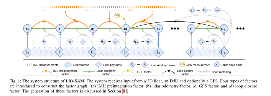
There are 4 types of factors in LIO-SAM: (a) IMU preintegration factors, (b) lidar odometry factors,(c) GPS factors, and (d) loop closure factors.

We denote the world frame as $\mathbf W$ and the robot body frame as $\mathbf B$. $\mathbf T_t^{\mathbf {BW}}$ is the transformation from world

IMU Preintegration

IMU will provide angular velocity and acceleration:

$$\begin{array}{l}\hat{\omega}_ {t}=\omega_ {t}+\mathbf{b}_ {t}^{\omega}+\mathbf{n}_ {t}^{\omega} \\\hat{\mathbf{a}}_ {t}=\mathbf{R}_ {t}^{\mathbf{B W}}\left(\mathbf{a}_ {t}-\mathbf{g}\right)+\mathbf{b}_ {t}^{\mathbf{a}}+\mathbf{n}_ {t}^{\mathbf{a}}\end{array}$$

where $\hat{\omega}_t$ (angular velocity) and $\hat{\mathbf{a}}_ {t}$ (acceleration) are the raw IMU measurements in $\mathbf B$ at time $t.$ $\mathbf b_t$ and $\mathbf n_t$are bias and white noise respectively. $\mathbf R_t^{\mathbf{BW}}$ is the rotation matrix from $\mathbf W$ to $\mathbf B$. $\mathbf g$ is the constant gravity vector in $\mathbf W$. And based on those measurements we could infer the motion of robot. The velocity, position and rotation of the robot at time $t + \Delta t$ can be computed as follows:

$$\begin{array}{l}\mathbf{v}_ {t+\Delta t}=\mathbf{v}_ {t}+\mathbf{g} \Delta t+\mathbf{R}_ {t}\left(\hat{\mathbf{a}}_ {t}-\mathbf{b}_ {t}^{\mathbf{a}}-\mathbf{n}_ {t}^{\mathbf{a}}\right) \Delta t \\\mathbf{p}_ {t+\Delta t}=\mathbf{p}_ {t}+\mathbf{v}_ {t} \Delta t+\frac{1}{2} \mathbf{g} \Delta t^{2}+\frac{1}{2} \mathbf{R}_ {t}\left(\hat{\mathbf{a}}_ {t}-\mathbf{b}_ {t}^{\mathbf{a}}-\mathbf{n}_ {t}^{\mathbf{a}}\right) \Delta t^{2} \\\mathbf{R}_ {t+\Delta t}=\mathbf{R}_ {t} \exp \left(\left(\hat{\omega}_ {t}-\mathbf{b}_ {t}^{\omega}-\mathbf{n}_ {t}^{\omega}\right) \Delta t\right)\end{array}$$

where $\mathbf{R}_ {t}=\mathbf{R}_ {t}^{\mathbf{W B}}=\mathbf{R}_ {t}^{\mathbf{B W}^{\top}}$. The IMU preintegrated measurements between time $i$ and $j$ can be computed as following (Apparently, $\Delta \mathbf{v}_ {i j}$ is not $v_j - v_i$ ):

$$\begin{aligned}\Delta \mathbf{v}_ {i j} &=\mathbf{R}_ {i}^{\top}\left(\mathbf{v}_ {j}-\mathbf{v}_ {i}-\mathbf{g} \Delta t_ {i j}\right) \\\Delta \mathbf{p}_ {i j} &=\mathbf{R}_ {i}^{\top}\left(\mathbf{p}_ {j}-\mathbf{p}_ {i}-\mathbf{v}_ {i} \Delta t_ {i j}-\frac{1}{2} \mathbf{g} \Delta t_ {i j}^{2}\right) \\\Delta \mathbf{R}_ {i j} &=\mathbf{R}_ {i}^{\top} \mathbf{R}_ {j} .\end{aligned}$$

See https://arxiv.org/pdf/1512.02363.pdf for detailed derivation.

Lidar Odometry

The lidar odometry in LIO-SAM is similar to Lego-LOAM or A-LOAM. The difference is LIO-SAM adopt keyframe strategy. When a new keyframe $\mathbb F_ {i}$ is registered, it will associate with a new robot state node $x_ {i}$ in the factor graph. The lidar frames between two keyframes will be discarded (Note that the position and rotation change thresholds for adding a new keyframe in LIO-LOAM are $1m$ and $10\degree$ respectively). The generation of a lidar odometry factor is described in the following step:

1. Sub-keyframes for voxel map. Organize $n$ most recent keframes as a sub-keyframes and combines their scans as a voxel map $\mathbf M_i = \left\{\mathbb{F}_ {i-n}, \ldots, \mathbb{F}_ {i}\right\}$, which includes edge feature voxel map $\mathbf M^{e}_i$ and plane feature voxel map $\mathbf M^{p}_i$. Note that $\mathbf M_i$ will be down-sampled to remove duplicated features.
2. Scan-matching. A new keyframe $\mathbb F_ {i+1}$ will be matched to $\mathbf M_ {i}$. The initial transformation $\tilde{\mathbf{T}}_ {i+1}$ is estimated through IMU. The matching process is similar to A-LOAM’s lidar mapping module.

GPS

System will still suffer from drift during long-distance navigation tasks. GPS is useful for correcting this long-distance-error. In LIO-SAM, a GPS factor is only added when the estimated position covariance is larger that the received GPS position covariance.

Loop Closure

LIO-SAM use a naive but effective method for loop closure detection based on the Euclidean distance. When a new node $x_ {i+1}$ is registered, we search for the near nodes from the factor graph. For example, $x_3$ is selected, and we match $\mathbb F_ {i+1}$ with the subkeframe voxel map $\left\{\mathbb{F}_ {3-m}, \ldots, \mathbb{F}_ {3}, \ldots, \mathbb{F}_ {3+m}\right\}$. If the matching succeed, a relative transformation $\Delta \mathbf T_ {3, i+1}$ will be added into fact graph as a loop closure factor. In LIO-SAM，$m = 12$ and the search radius is $15m$.